We celebrated New Year’s Eve with our traditional time travel movie. This year’s picks were a Keanu Reeves double feature: The Lake House and the classic Bill and Ted’s Excellent Adventure. Be excellent to each other!
Happy New Year!
We celebrated New Year’s Eve with our traditional time travel movie. This year’s picks were a Keanu Reeves double feature: The Lake House and the classic Bill and Ted’s Excellent Adventure. Be excellent to each other!
Happy New Year!

NGC6888, also called the Crescent Nebula, is an emission nebula around a Wolf-Rayet Star, WR136. It’s located in the Milky Way, approximately 5000 light years away, and it has an apparent size of 18 x 12 arcminutes, making it 26 x 17.5 light years across. It’s estimated to be 30,000 years old.
Although it may seem similar since it is a nebula around a star, the Crescent Nebula is not a planetary nebula, and its ultimate ending will be very different from a planetary nebula. Planetary nebulae occur when an intermediate mass star, 1 to 8 solar masses, expands into a red giant, sheds its outer layer, and shrinks to a white dwarf. The high temperature and wind from the white dwarf ionizes the shed outer layer, making the beautiful nebulae. The Crescent Nebula was made by a massive star, estimated to initially be <= 50 solar masses. When it was a main sequence star, fusing hydrogen early in its life, its solar wind blew a bubble in the gasses surrounding it. When it became a Red Super Giant, its slow solar wind filled the bubble with its outer layer, estimated to be 25 solar masses worth of material. And when the star collapsed into a super hot Wolf-Rayet star, now about 21 solar masses in size, its fast solar wind compressed the red super giant and Wolf-Rayet material into ionized filaments and clumps. Eventually, the Wolf-Rayet star will fuse its matter creating heavier and heavier elements until it reaches iron, when it will implode and create a supernova.

Visually, the nebula appears to have an outer Oiii “skin” and a “clumpy” Ha interior. The Oiii skin is the boundary between the main sequence bubble and the Wolf Rayet shell, and the clumpy Ha interior is the red super giant material compressed by the Wolf Rayet shell. A “blowout” in the Oiii skin can be seen in the lower right in the blue Oiii in this image. The Interstellar Medium (ISM) – the cold low density gas between stars – may have been less dense in this direction, allowing the Oiii skin to blow out in this direction and not in other directions where the ISM is denser.
I used data from my driveway in Friendswood, Texas with suburban Bortle 7 – 8 brightness skies (lots of light pollution) to make this image. In order to capture the detail in this nebula and the outer Oiii shell, I needed a lot of data: 12.4 hours of Ha data and 15 hours of Oiii data, plus an hour of RGB data for the stars, taken over ten nights.
This is a narrowband image, mapping Oiii to blue and Ha to red. My goal was to capture both the details in the Ha and the outer Oiii shell.
Some people think this looks like a cosmic “brain.” What do you think? Isn’t our galaxy beautiful?
Camera geek info – Narrowband:
Frames:
Processing geek info:
Comet C/2023 Tsuchinshan ATLAS looped around the sun on September 27, 2024 and started on its path back towards the outer solar system. For a few days, it was not visible because it was too close to the sun. But it was predicted to become visible again around October 11, and it would be the closest to the Earth on October 12, 2024.
We were in Dell City at the time and staked out a sunset viewing spot with a long view to the west.
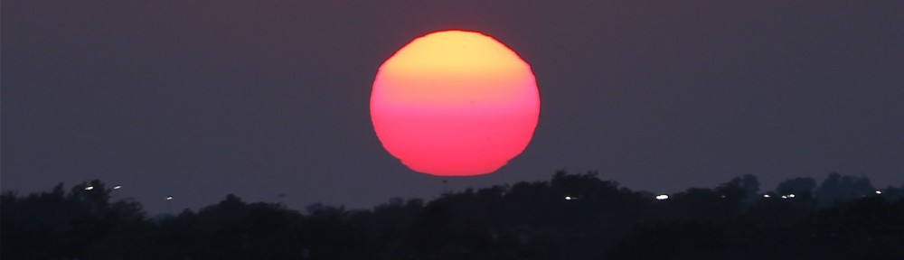
We made our first attempt to see the comet on October 10, 2024. The comet should have been barely above the horizon at sunset, and unless it was truly extraordinary, we were unlikely to be able to see it. We were treated to a lovely sunset, but we could not spot the comet. I had told myself this was a dry run, so I wasn’t too disappointed. And, when we returned back to our B&B, we were treated to a rare viewing of the northern lights from Texas.
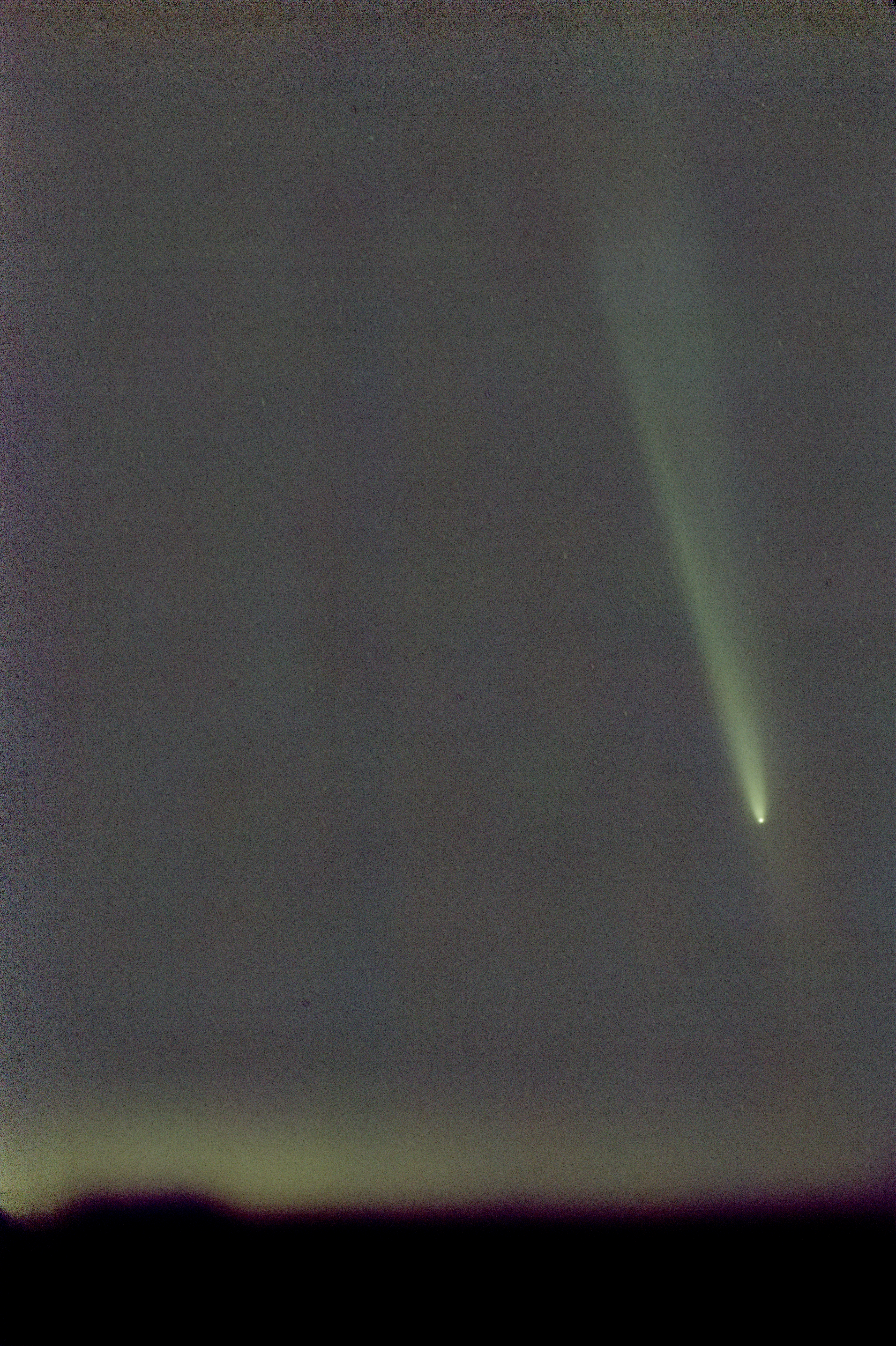
We made a second attempt to see the comet on October 11, 2024. The comet was supposed to be higher above the horizon at sunset than the day before. There were low clouds in the sky. We saw a lot of “fake comets” – bright airplane contrails. Eventually my husband found the comet with his binoculars – success! I started taking pictures, but I hadn’t used the right settings, and when I discovered that later, I suspected that the data would not be usable. I was right – I can see a moving smudge in the images, but it’s not good enough for PixInsight to comet align the images (and there aren’t enough stars in the images for it to star align them).
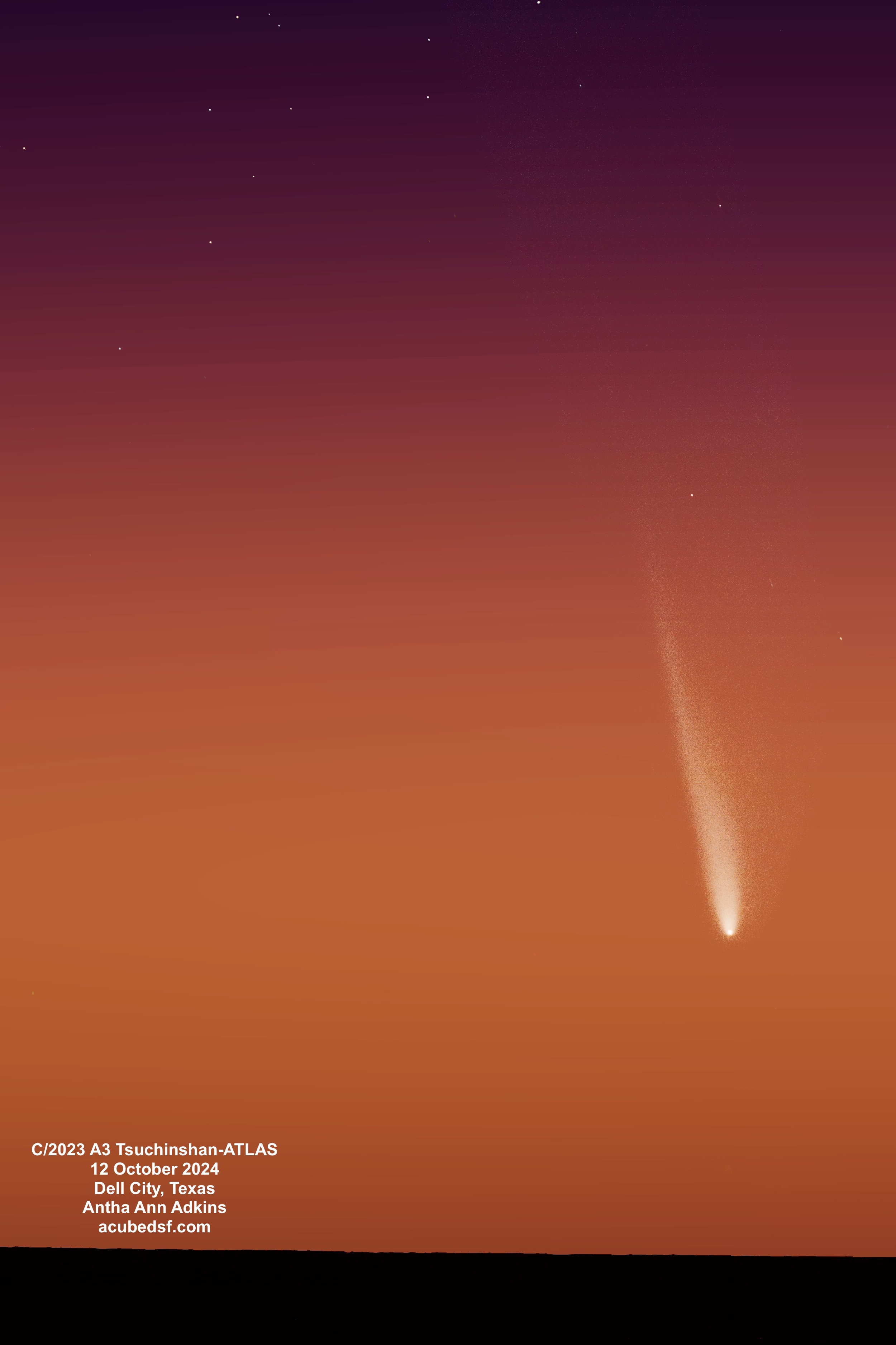
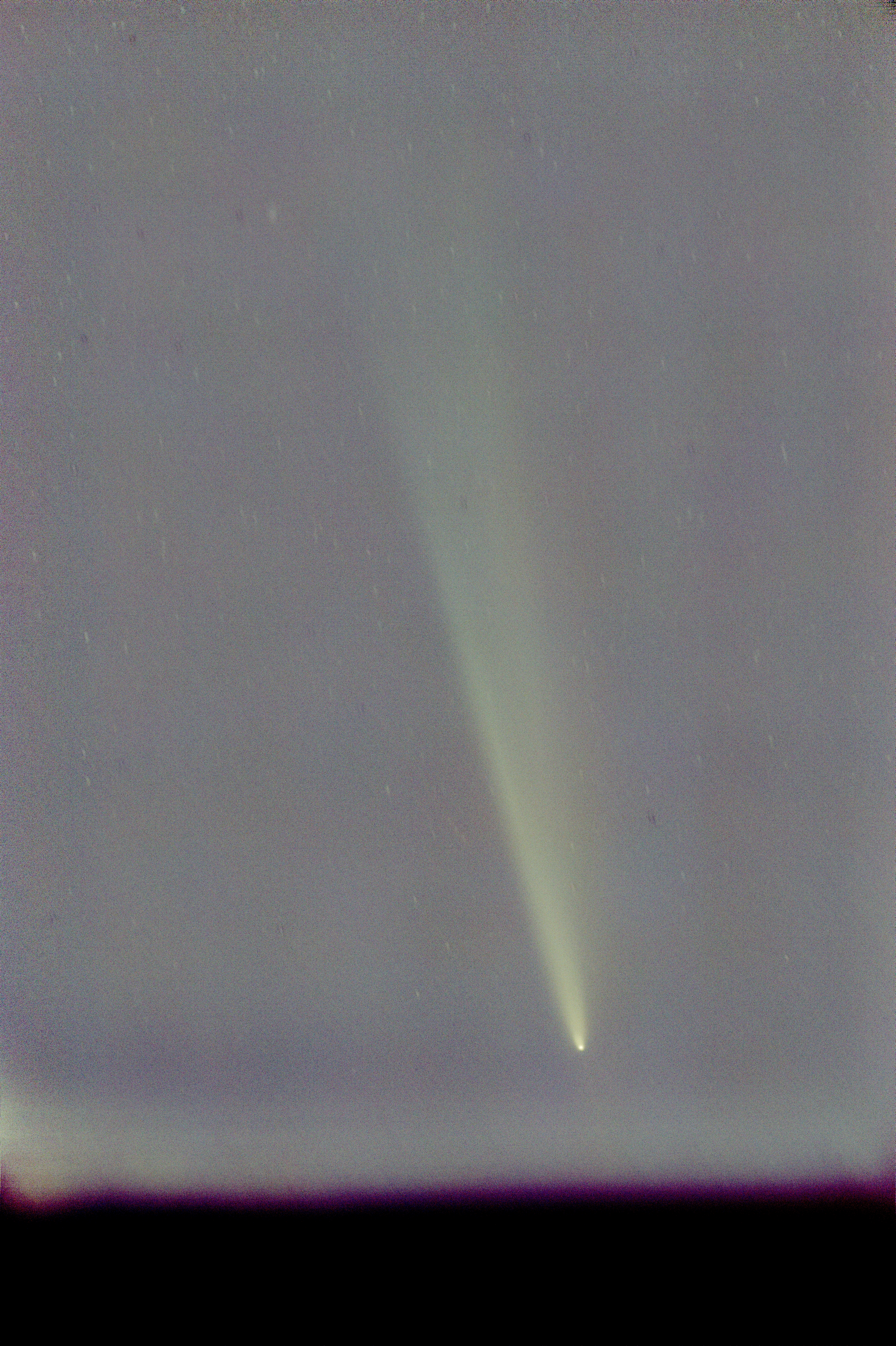
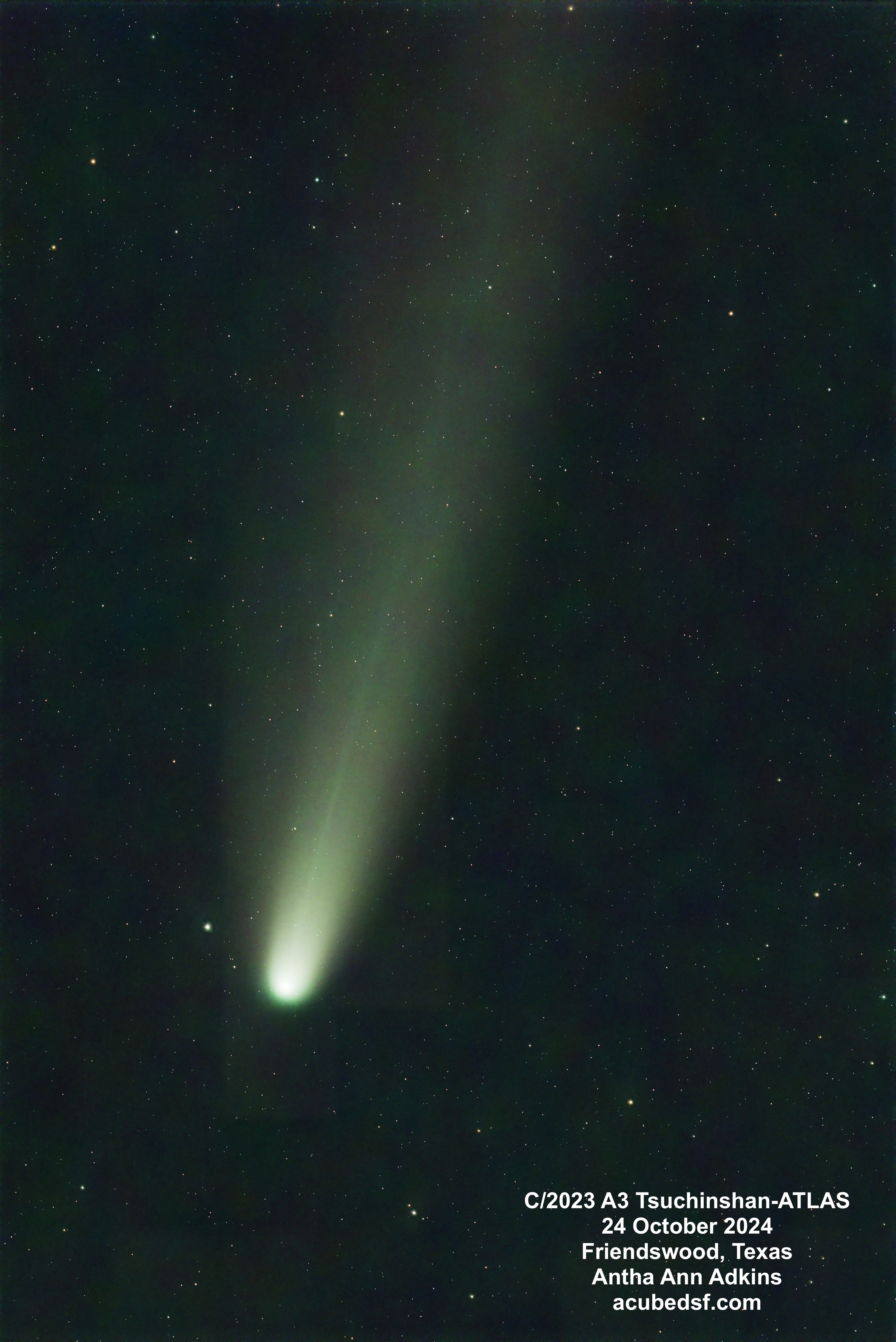
We made a third attempt – third time is the charm! – on October 12, 2024. The comet was supposed to be more than 10 degrees above the horizon at sunset, and it had been the closest it would be to the Earth, 0.47239 AU or 70668538.14 km, just nine hours earlier. This time there weren’t any clouds. And this time we could easily find the comet and see that it had a huge tail! Given my experience the night before, I made sure I was using good camera settings, and I could see the comet and its tail in single images.
I used PixInsight to stack 50 images (8.3 minutes of data) to make this final image – my first post-solar-swing image of C2023 A3. Isn’t it beautiful?
Today, on this day of Thanksgiving, I am most thankful for my family and friends, near and far. But I’m also thankful for all the wonder to be found in this universe we live in, and particularly for this comet. Happy Thanksgiving!
Camera geek info:
Frames:
Processing geek info:
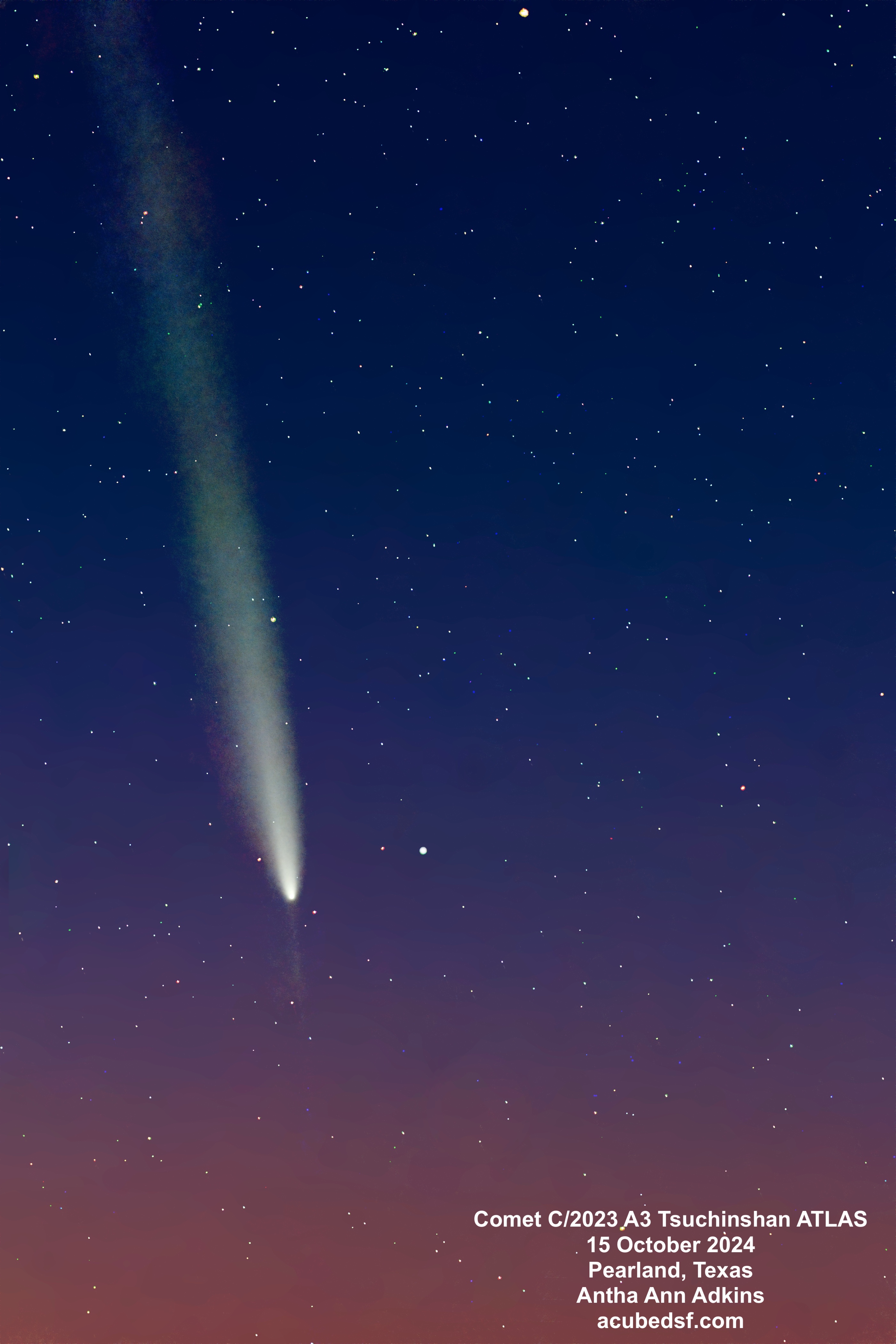
Our last visit to Dell City, Texas ended with a fun event: going comet hunting with new friends.
I knew from comet hunting with my husband the previous evening that C/2023 A3 Tsuchinshan-ATLAS would be visible in the early evening sky. But this time, I wanted to image it over the Cornudas Mountains to the west of town. I also wanted to have a view over the flat fields to the mountains and the sky above – which I could find by driving just a few blocks north of the center of town.
I invited some new local friends to join us, and they came in a pickup truck loaded with lawn chairs. It was a comet tailgate party!
We had a great time visiting while we watched the sky as Venus appeared, followed by some bright stars, followed by the comet. We could see it naked eye! We could even see the comet’s tail naked eye! It was pretty impressive.
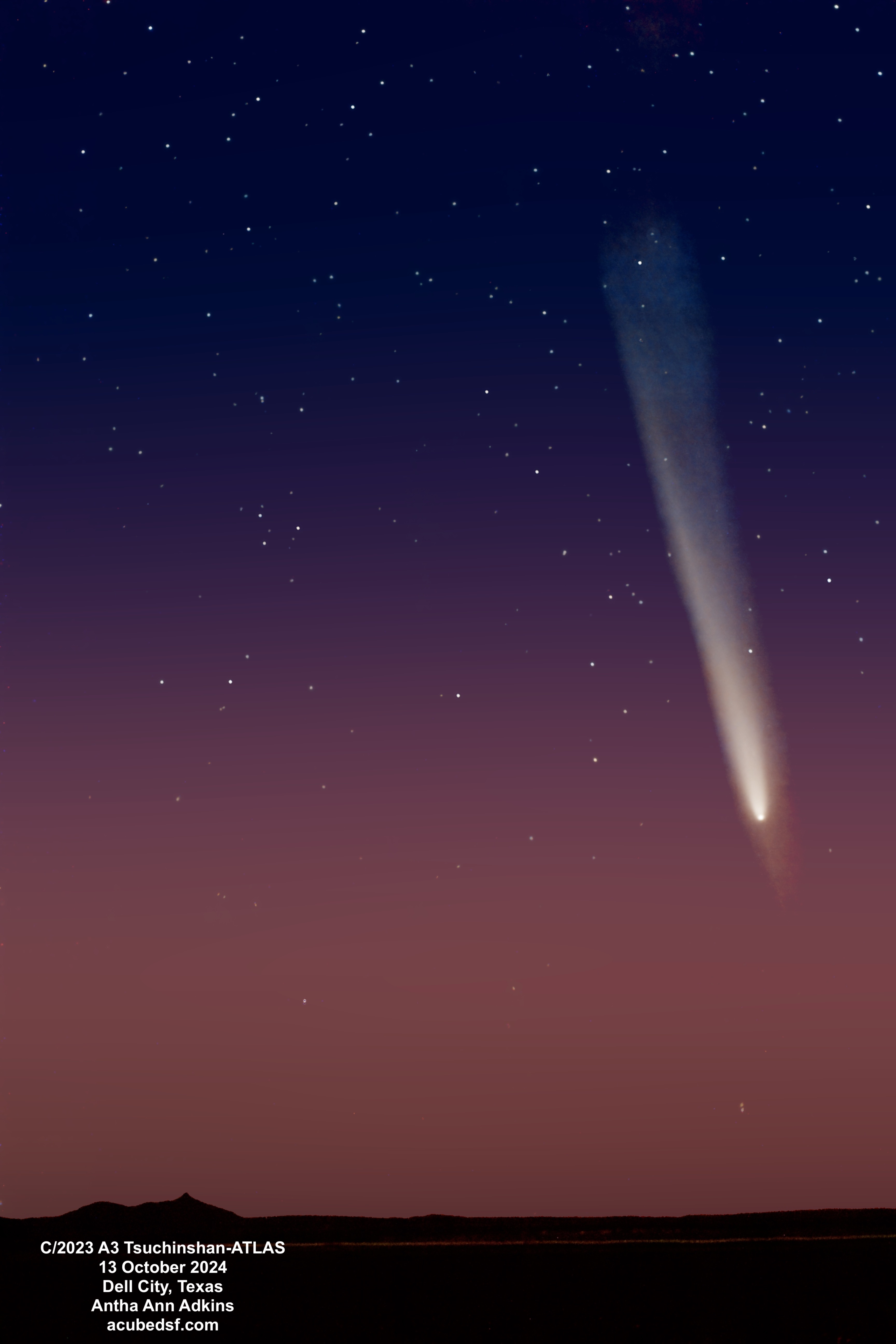
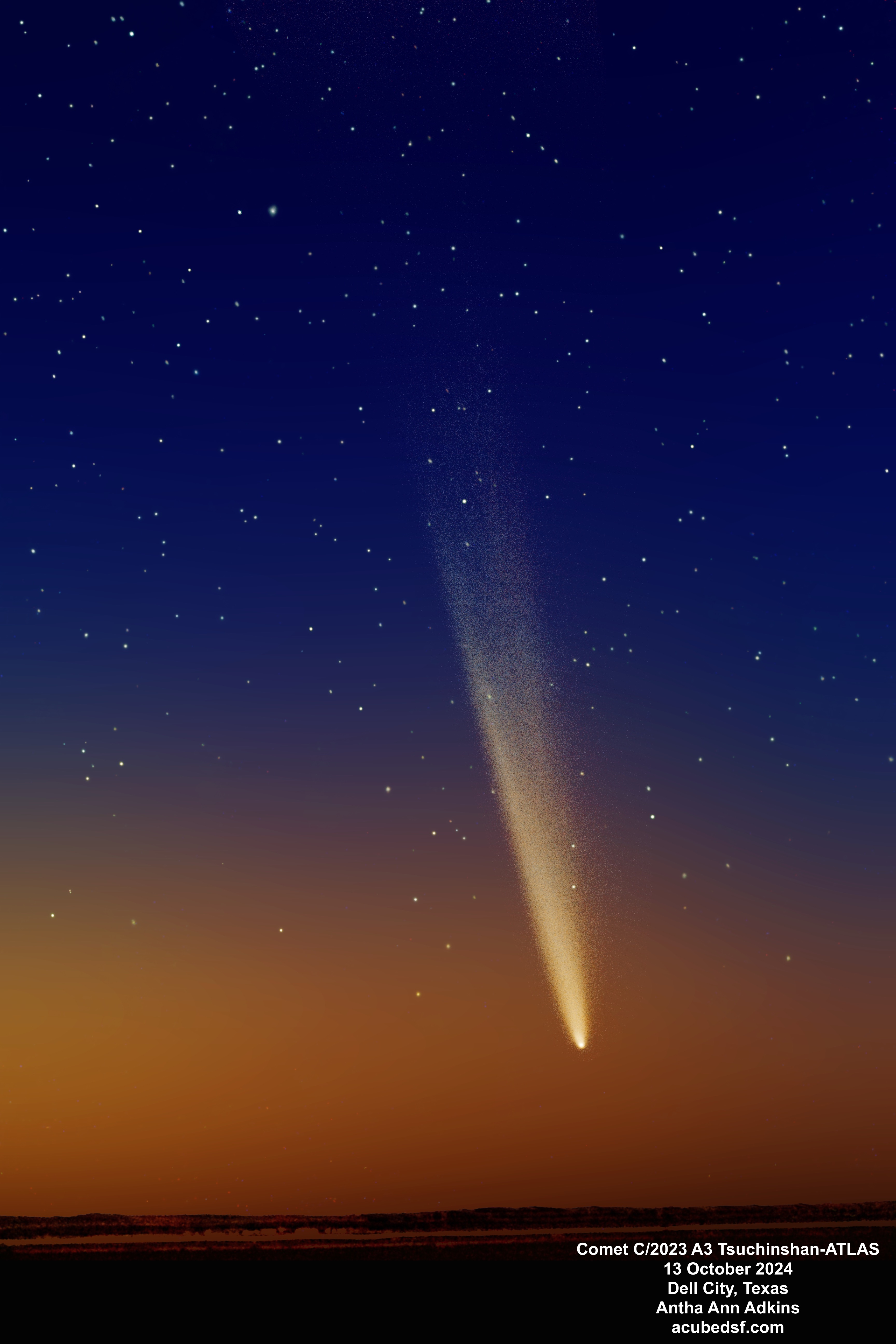
It’s taken me over a month to learn how to and successfully process these pictures. Each picture used one set of images for the comet, stars, sky, and foreground/mountains, but each part was processed separately. The earlier pink picture where the comet is higher in the sky was made from 120 4 second shots (8 minutes of data). The later orange picture where the comet is lower in the sky was made from 75 10 second shots (12.5 minutes of data).
One of the things I tried to do while processing was to make sure that all the fuzz around the comet and the anti-tail were real and not processing artifacts. You can use the sliders below to compare the final images with the comet-only portion to see that, if anything, the final images show less fuzz than what was in the data. (The comet-only data was calibrated, blur exterminated, star exterminated, comet-aligned, stacked, dynamic background extracted, and stretched.)
This event is high on my list of “coolest astro things I’ve seen.” And I’m glad I had such a great group of folks to share it with.
What cool things have you shared with friends recently?
Camera geek info:
Frames:
Processing geek info:
Comet C/2023 A3 Tsuchinshan ATLAS put on quite a show after it rounded the sun and passed by the Earth on its way likely out of our solar system. With an orbital eccentricity greater than 1, its orbit appears to be hyperbolic, meaning it’s not coming back unless something perturbs its orbit.
In this picture, you can see the comet’s bright nucleus and coma, its long dust tail, and its anti-tail, but not a separate ion tail.
When comets travel close to the sun, solar radiation heats up the comet nucleus, and it outgasses. Outgassing delivers both gas and dust to the region around the nucleus, forming a coma, a (temporary) atmosphere around the comet. The solar radiation and solar wind act on this coma to push the gas and dust away from the sun to form a tail. Three separate tails can be visible: the ion tail, the dust tail, and the anti-tail. The ion tail, also called the gas tail or type I tail, is the tail formed by the ionized gasses pushed away from the comet, and it points away from the sun. The dust tail, also called the type II tail, is the tail formed by the dust pushed away from the comet, and it stays more in the comet’s orbit and appears to curve away from the gas tail. The anti-tail consists of the larger dust particles that were not pushed as much and remained in the comet’s orbit. The anti-tail appears to point towards the sun, and it is only visible when the Earth passes through the comet’s orbital plane near the time when the comet passed by the sun. Because of these special conditions to see the anti-tail, it is not observed with most comets.
Another item visible in the image is M5, a globular cluster in our galaxy. It is the large bright “star” to the right of the comet nucleus. Because this image was taken with an 85 mm lens, and M5 was sorted to the “stars” image in my processing, it just appears to be a large bright star. I suspect with some additional processing, I could have made it look fuzzier, though there aren’t a lot of pixels at this scale. The Messier objects are “fuzzy” objects that comet-hunter Charles Messier made a list of because they weren’t comets – so it’s fun to see one next to a comet. M5 is 24,500 light years away from Earth and has an angular size of 23 arc-minutes, making it about 165 light years across. It’s thought to be one of our galaxy’s older globular clusters, at 13 billion years old.
Processing this image was tricky for several reasons: 1) it was made from images taken with a camera on a tripod, so the sky was moving in each frame, 2) the comet was moving relative to the sky, and 3) the images were taken at dusk, when the sky gradient is also changing in every image. I benefited greatly from following the methods and advice in Adam Block’s Comet Academy. One additional trick I used was to run BlurXterminator in correction only mode on all the registered images as my first step since the 4 second tripod images had visible star trails.
Getting to this image has taken almost a month of watching videos, learning new tools, and trying various tool combinations and settings. Some of these steps had to be run on each individual image – all 233 of them – meaning some processing steps took many hours. After all that work, I am happy with the results.
I started with this image because I thought it would be the easiest of my set of C2023A3 comet images to process … the other images are from darker skies in terms of light pollution but closer to dusk and include a foreground. But the comet was brighter! I’m really looking forward to processing them and sharing the result! Hopefully they won’t take a month each to process!
Camera geek info:
Frames:
Processing geek info:
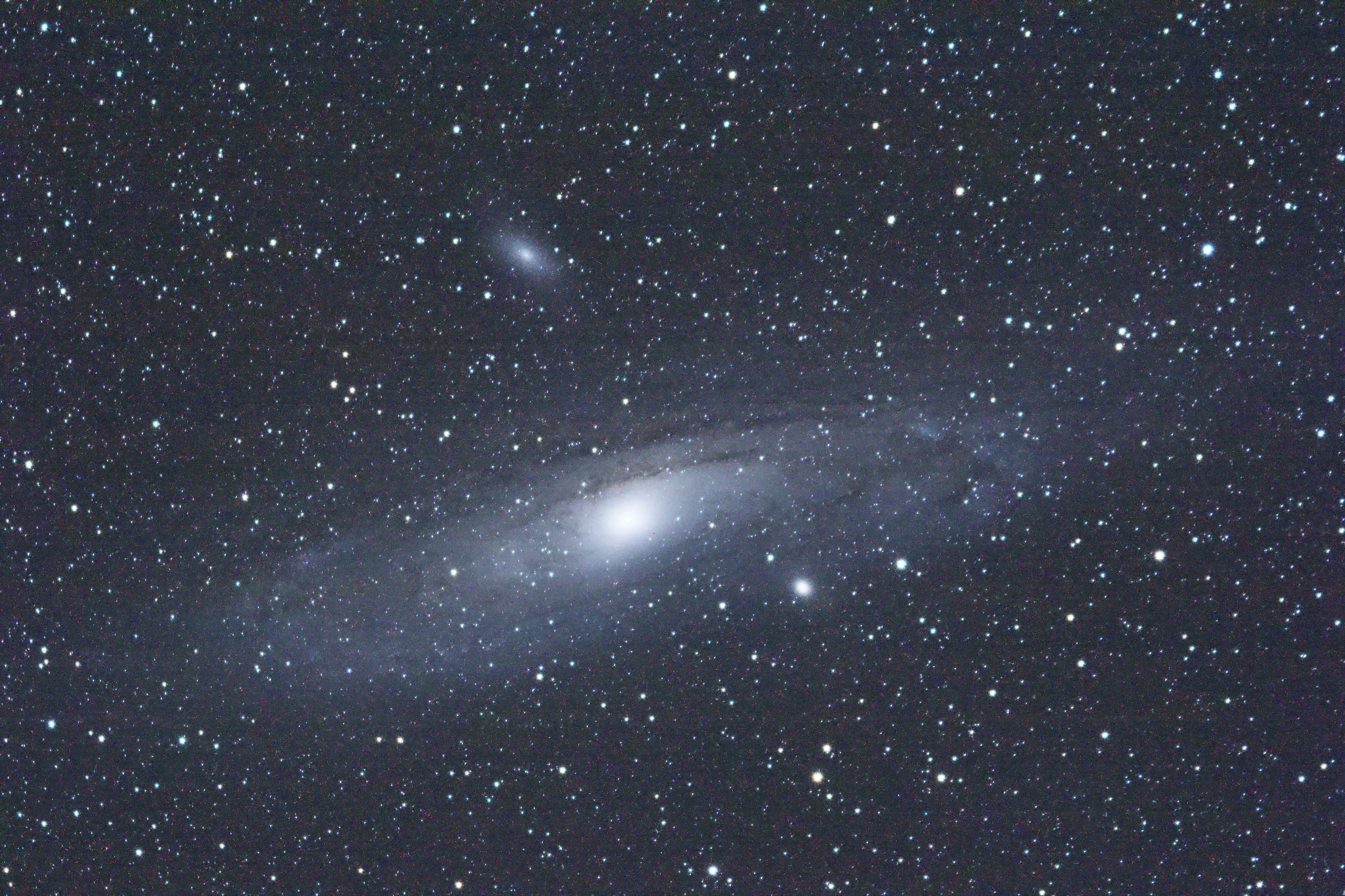
The first object that I got a satisfactory image of with my tracking mount and telescope and DSLR was M31, the Andromeda Galaxy, from the dark skies of Dell City, Texas in October 2022. My first image, above, was a 3 minute long exposure. I was so excited to have a good image that I took a picture of my camera’s viewfinder to send the picture to people.
When I came home to Friendswood, Texas, I did some experiments to see if I could get the same results. It was not a surprise when the answer was “no” – my home skies are much more light polluted – I expected to get a completely white screen and was surprised when I could still see a hint of the galaxy.
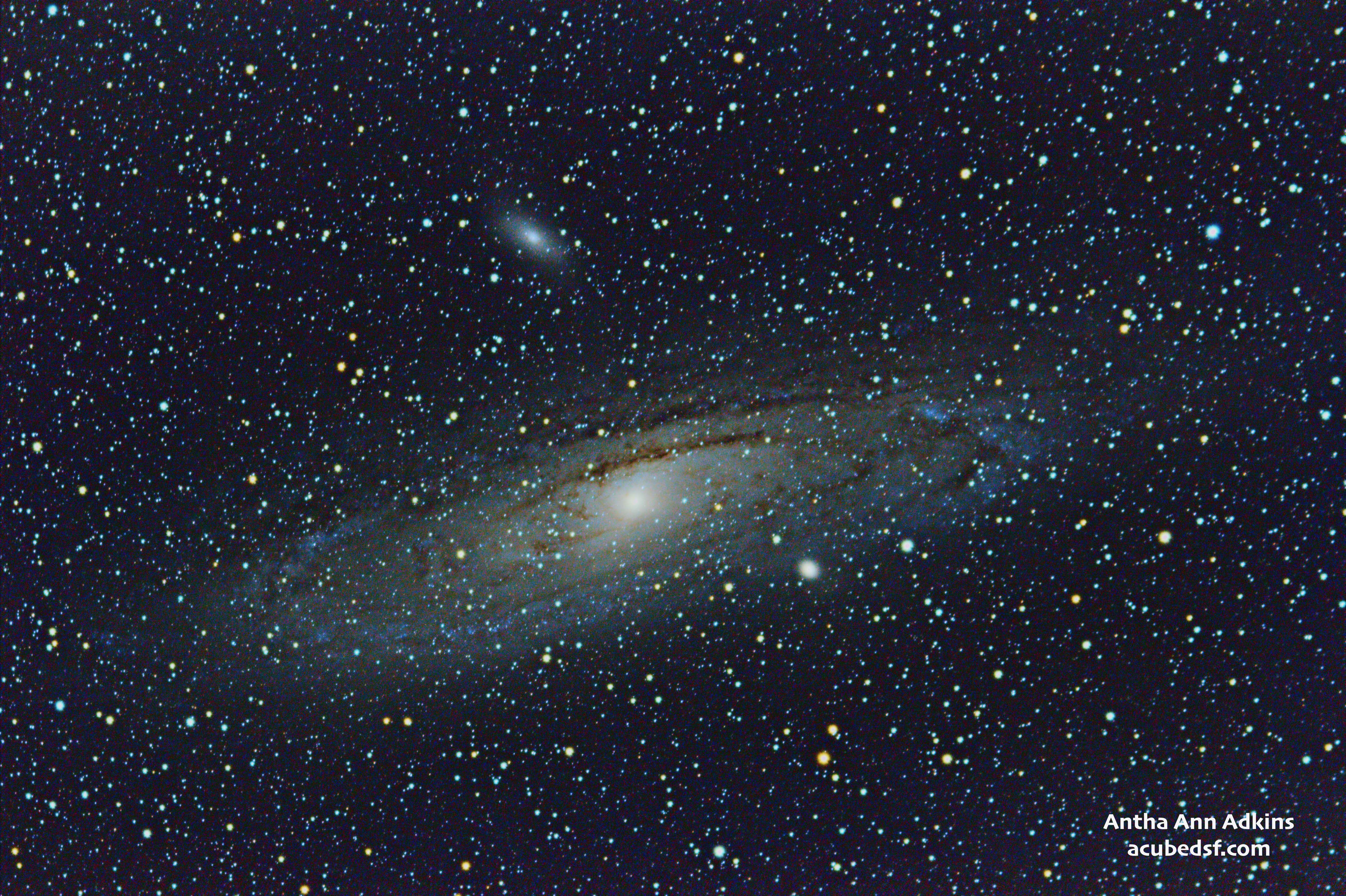
I started to learn how to use PixInsight, a powerhouse astrophotography processing tool, in the winter of 2022. I learned enough to be able to stack 18 3 minute images to make my Christmas card photo and the picture I am still using as my computer background at work.
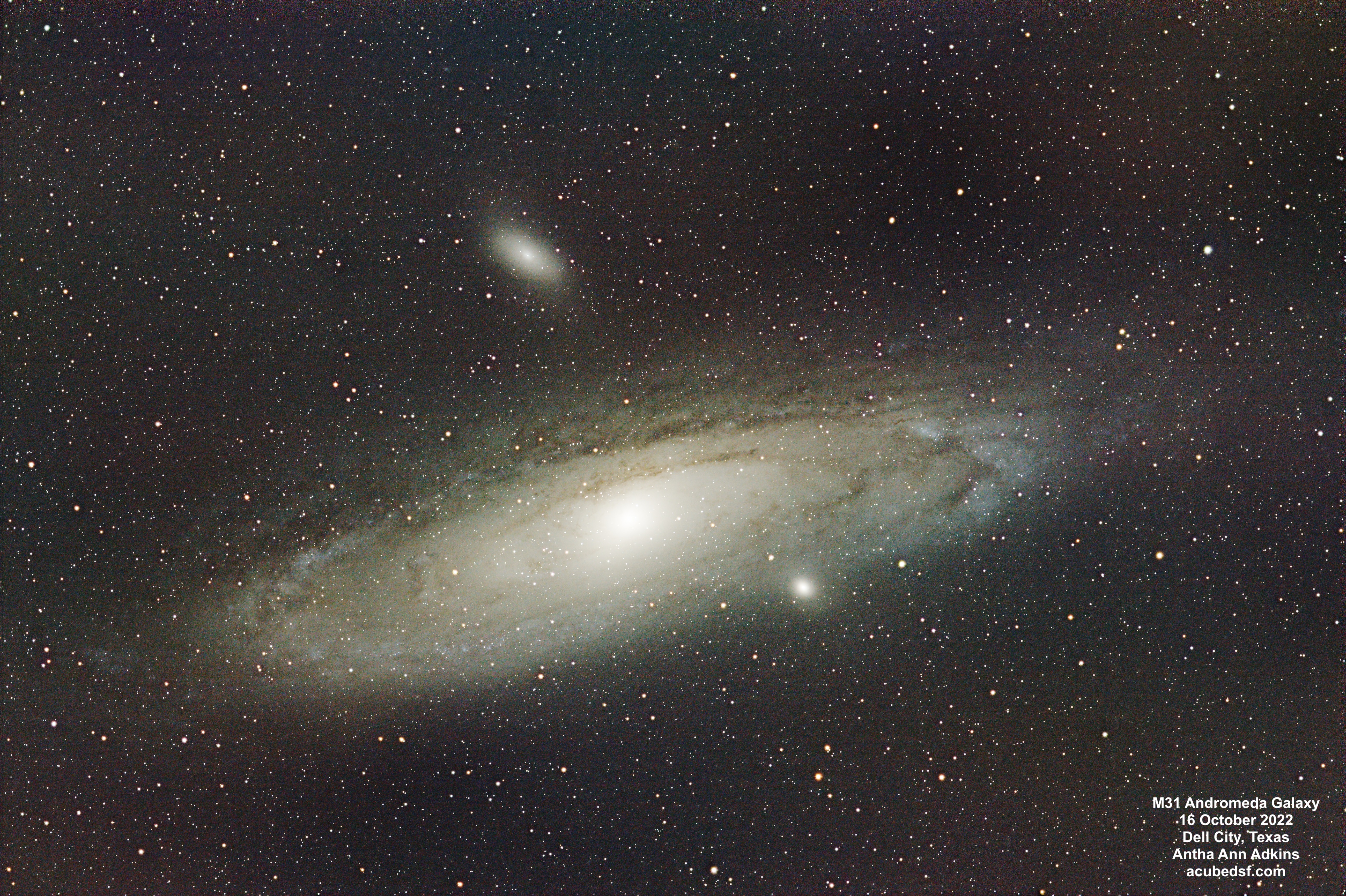
I’ve learned a more about astrophotography processing since then, most notably adding Russ Croman’s excellent BlurXterminator, NoiseXterminator, and StarXterminator tools to my toolbox and learning a ton from Adam Block’s videos. So I reprocessed the data above using my current knowledge and toolset.
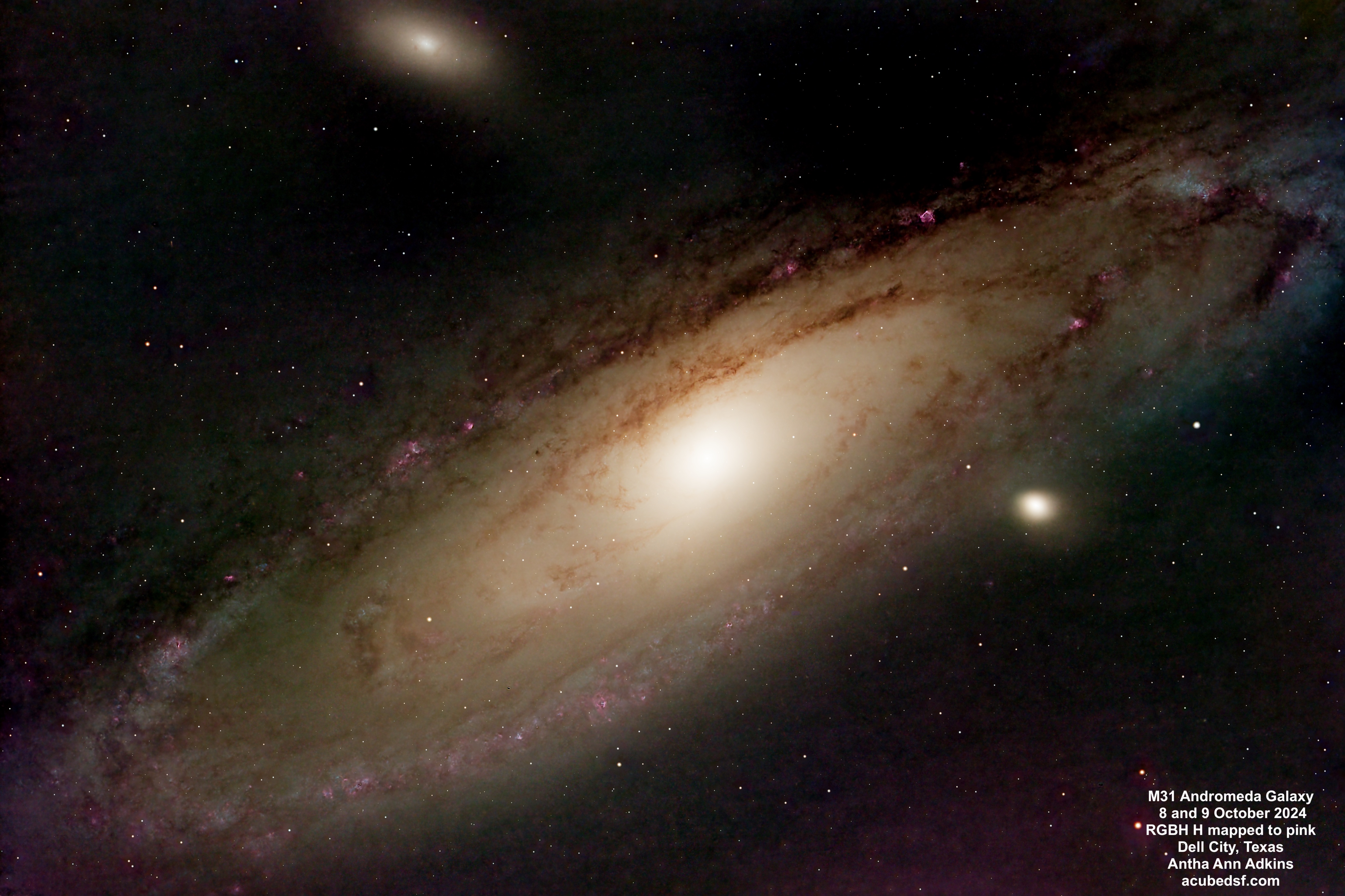
Finally, in October 2024, we were back in Dell City, and I collected new M31 data using an astrocamera and red, blue, green and hydrogen-alpha filters. I had to learn more in order to be able to merge the Ha data into the RGB data. Luckily, there are Adam Block’s videos! One new trick I had to use was “continuum subtraction” – removing the background red from the stars from the Ha data.
Sometimes, when other things aren’t working out (comet processing), it’s good to step back and see how far you’ve come. I’ve learned a lot over two years … and I’m looking forward to learning a lot more!
What are you learning about?
When we travel to the fabulous dark skies of Dell City, Texas, I try to pick a combination of challenging targets and targets that I’m confident I’ll get good results with. In October, one of my picks for the “good result” target was M31, the Andromeda Galaxy.
It seemed fitting to image the Andromeda Galaxy now because we are approaching the 100 year anniversary of Dr. Edwin Hubble’s November 23, 1924 New York Times article confirming that some objects classified as nebulae were, in fact, “island universes” – galaxies separate from our own. Hubble used the Cephid variable stars in the Andromeda Galaxy and in M33 to measure the distance to those two galaxies and determine that they had to be outside of our own galaxy – on the order of 1 million light years away. Based on that distance and its apparent size, Hubble calculated that the Andromeda Galaxy’s diameter was 45,000 light years.
100 years later, the Andromeda Galaxy is known to be 2.56 million light years away. Its apparent size is 3.167 degrees by 1 degree, giving it a diameter of 141,000 light years. So even further and even bigger than Hubble calculated!
It is amazing to me that we’ve only understood that there were other galaxies for 100 years! And I think it is cool that we keep learning more and more about the universe around us.
This image of the Andromeda Galaxy was captured using red, green, blue and hydrogen-alpha filters. Although Ha actually is in the red part of the spectrum, it is frequently mapped to purple-pink so it stands out, and I have used that mapping here. These Ha regions are star-forming nebula in the Andromeda Galaxy, similar to our own Orion nebula and Eagle Nebula.
So while Hubble proved that Andromeda was a galaxy and not a nebula … it also contains its own nebulae. And we can see them! How amazing is that?
Camera geek info:
Frames:
Processing geek info:
I have a bunch of wide field comet images from Dell City, Texas and Pearland, Texas that are proving … challenging … to process, given that they were taken near dusk with a DSLR on a tripod. Everything is changing – the Earth is rotating (so the stars are moving relative to the camera on a non-tracking tripod), the comet is moving relative to the stars, and the sky brightness is changing.
But now Comet C/2023 A3 Tsuchinshan Atlas is getting higher in the night sky, so it is no longer visible only at dusk. So I could set up my tracking mount and telescope to image it. The tail is still really long – much longer than I can capture in the field of view of my telescope!
Even with a tracking mount and dark sky, processing a comet moving relative to the stars is still really challenging, and I really benefited from following the “Standard Comet” example in Adam Block’s Comet Academy.
Camera geek info:
Frames:
Processing geek info:
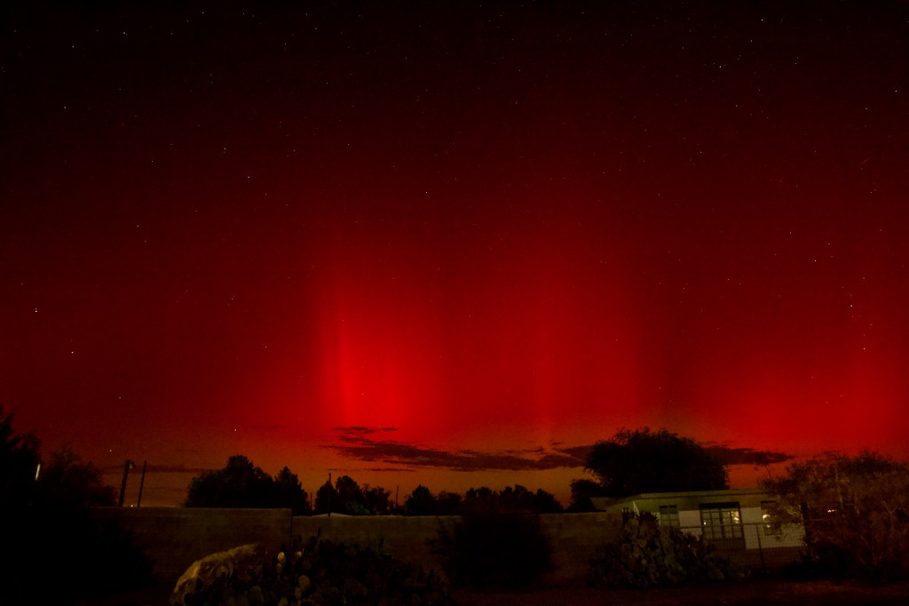
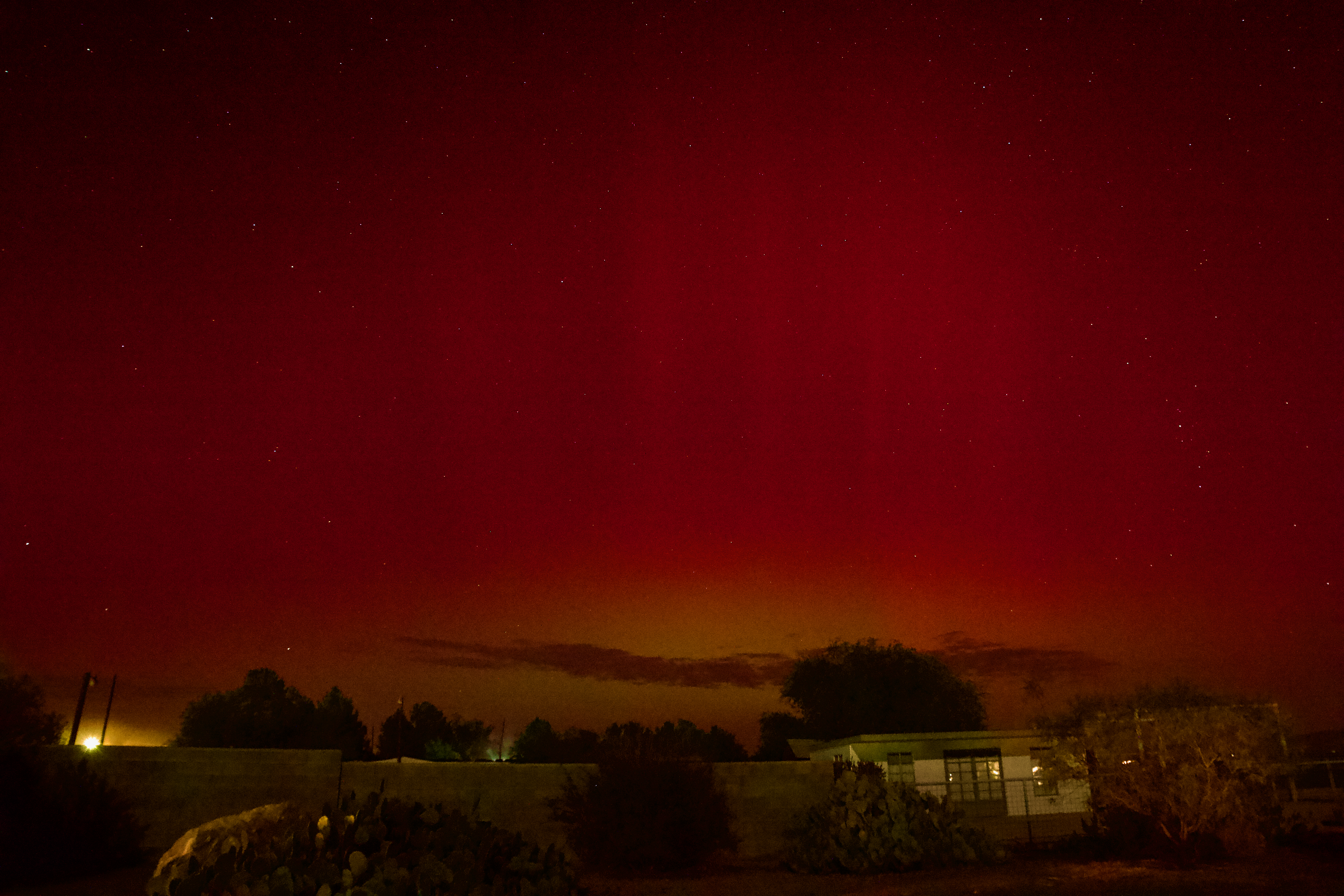
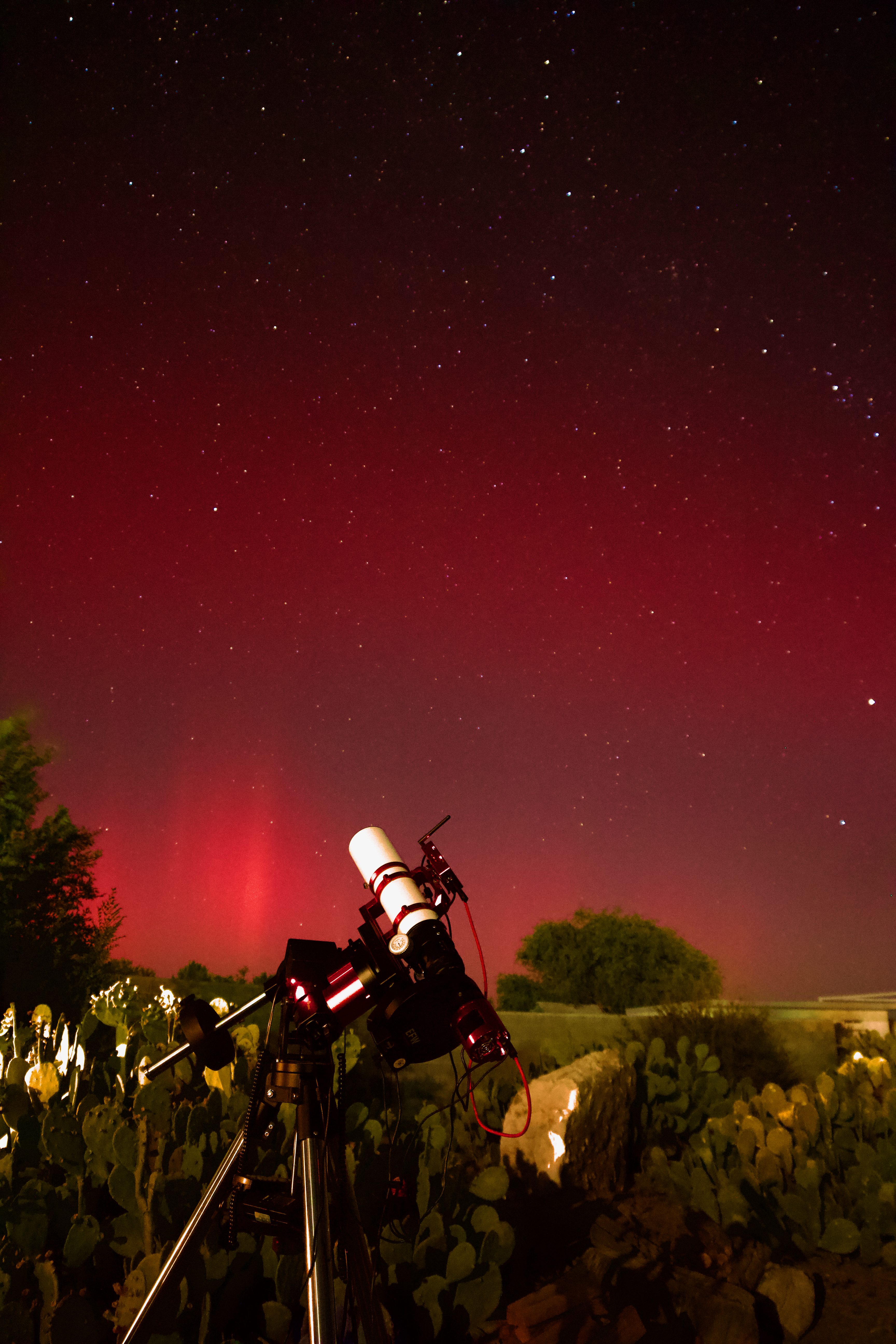
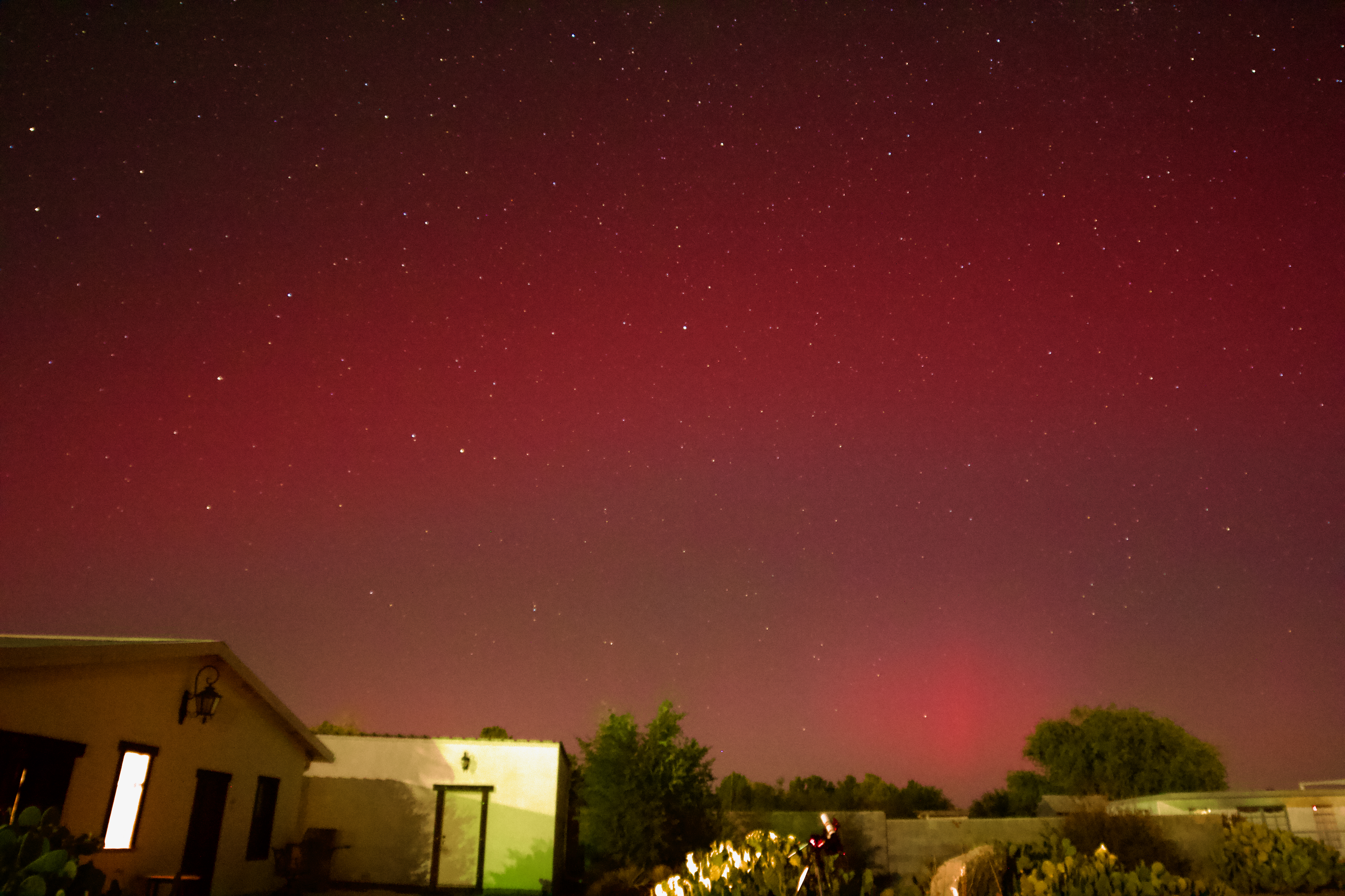
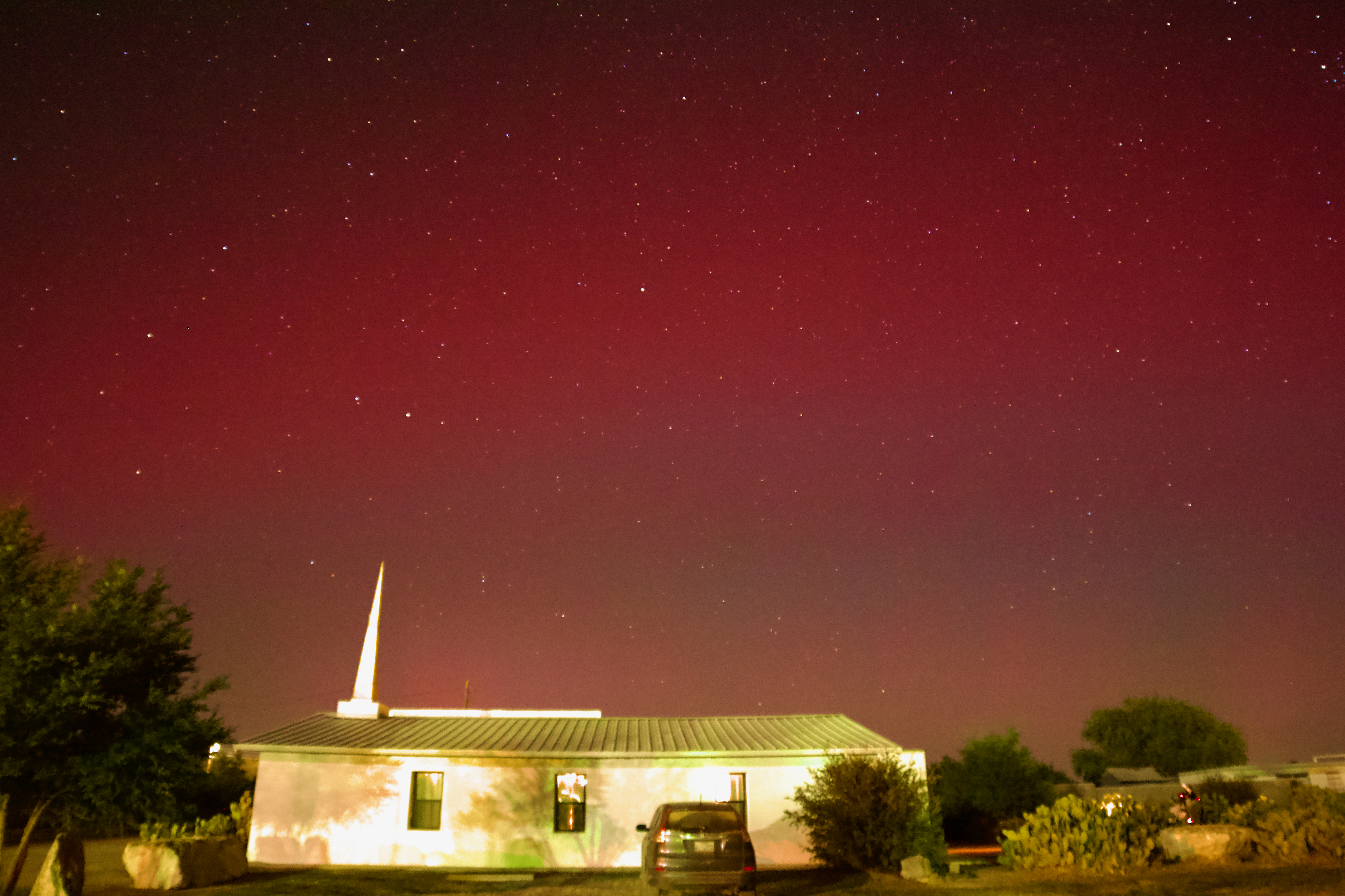
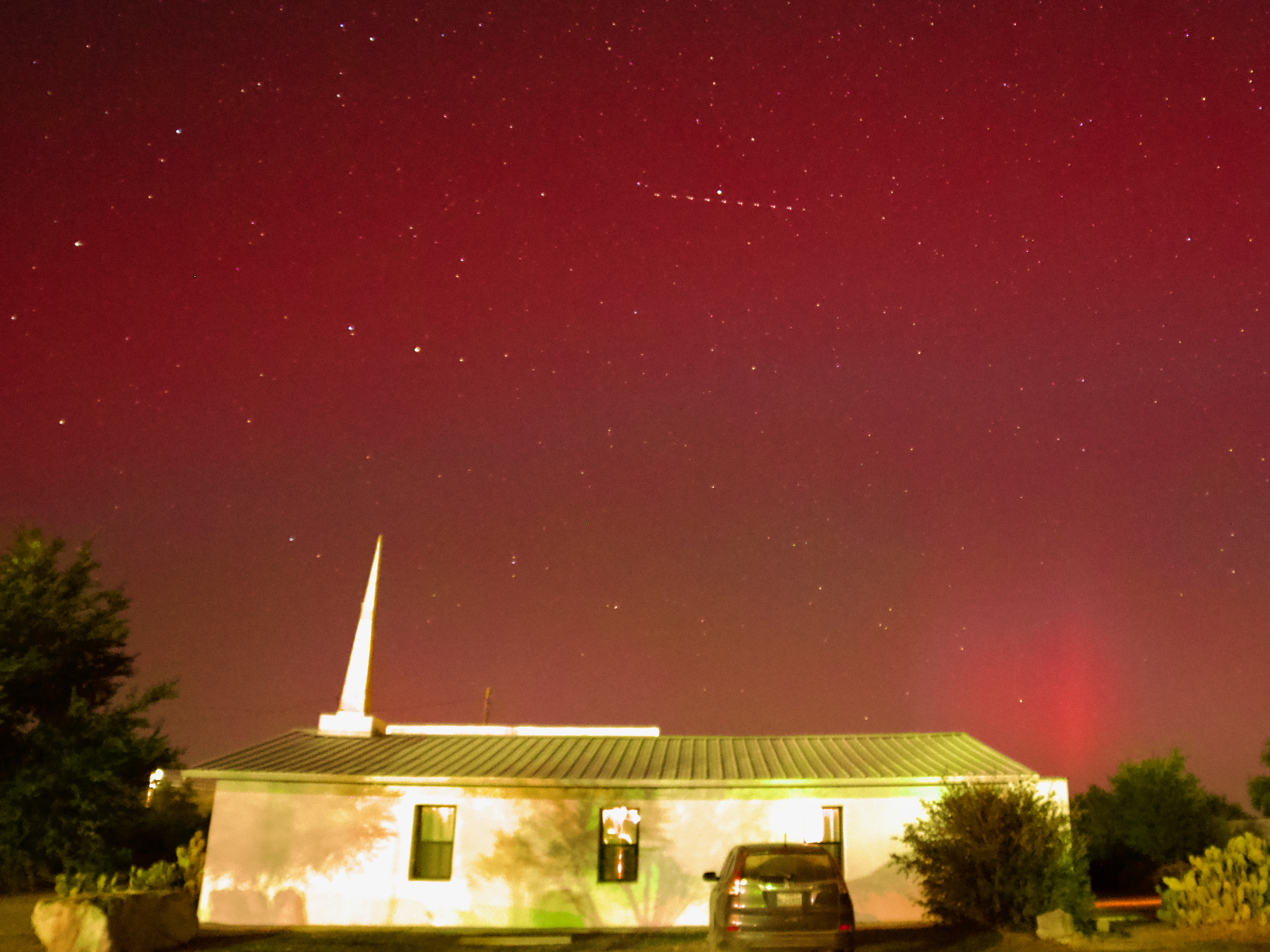
Earlier this month, we were very lucky and happened to be at my favorite dark sky site – Dell City, Texas – when I got an alert on my phone that we might have a Kp8 geomagnetic storm coming the next day, with a chance to see the Northern Lights much lower than usual.
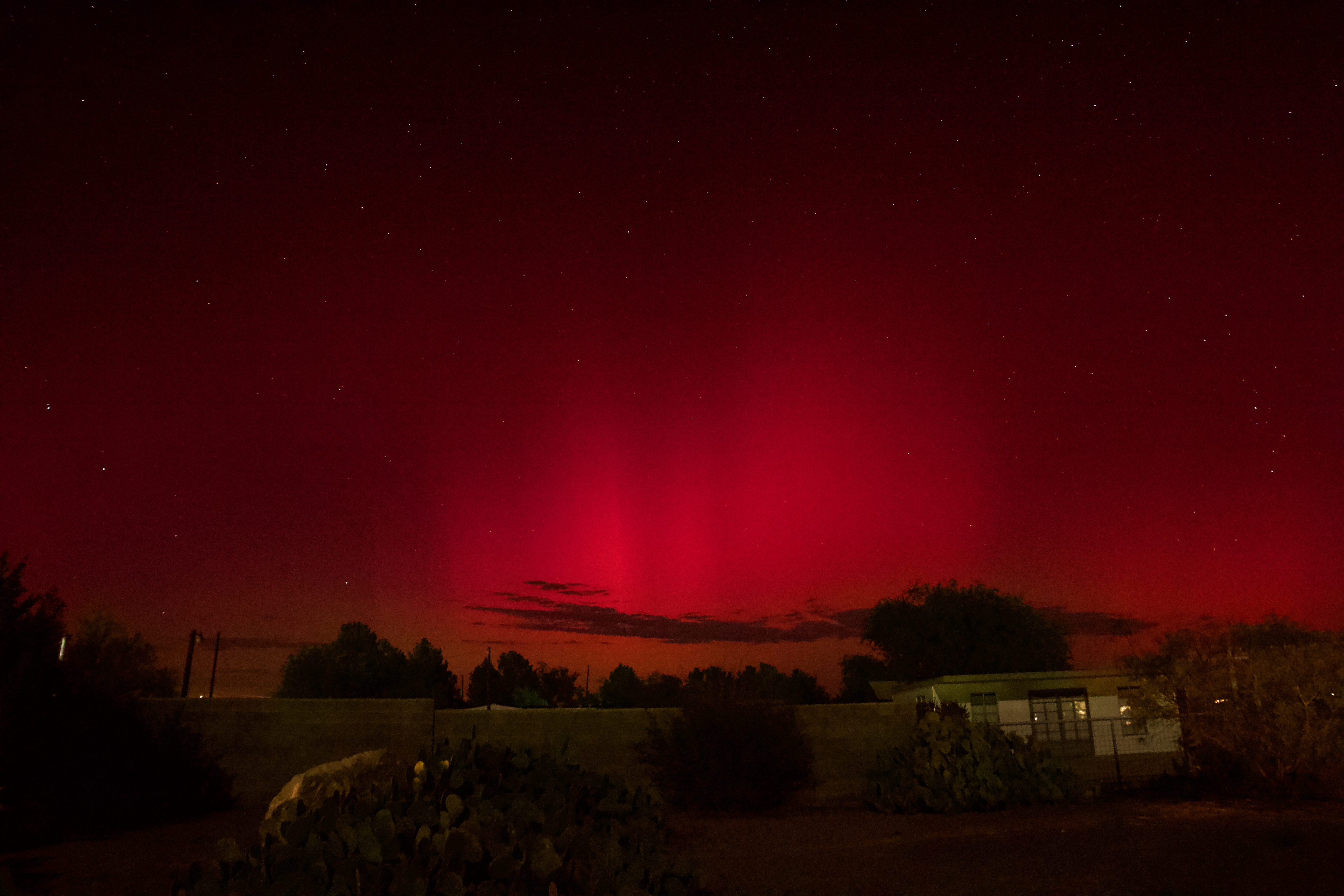
I have the app on my phone because we’ve traveled to places where seeing the Northern Lights was possible. We even saw them on the horizon from Inverness, Scotland. We’ve also been on two trips where Northern Lights tours were on the agenda – but both tours were cancelled due to weather. Earlier this year, when there was another big geomagnetic storm, we went north to Conroe, Texas where people reported seeing the lights. I found a great foreground – but alas, no lights.
So imagine my delight when I was setting up my telescope in Dell City, Texas, where the skies are very familiar to me, and I looked up and saw moving red lights to the north. Red lights to the north are not normal. The Northern Lights were visible from Texas! I literally sprinted into our Air B&B to get my husband and my camera.
I took glamour shots of my telescope with the aurora.
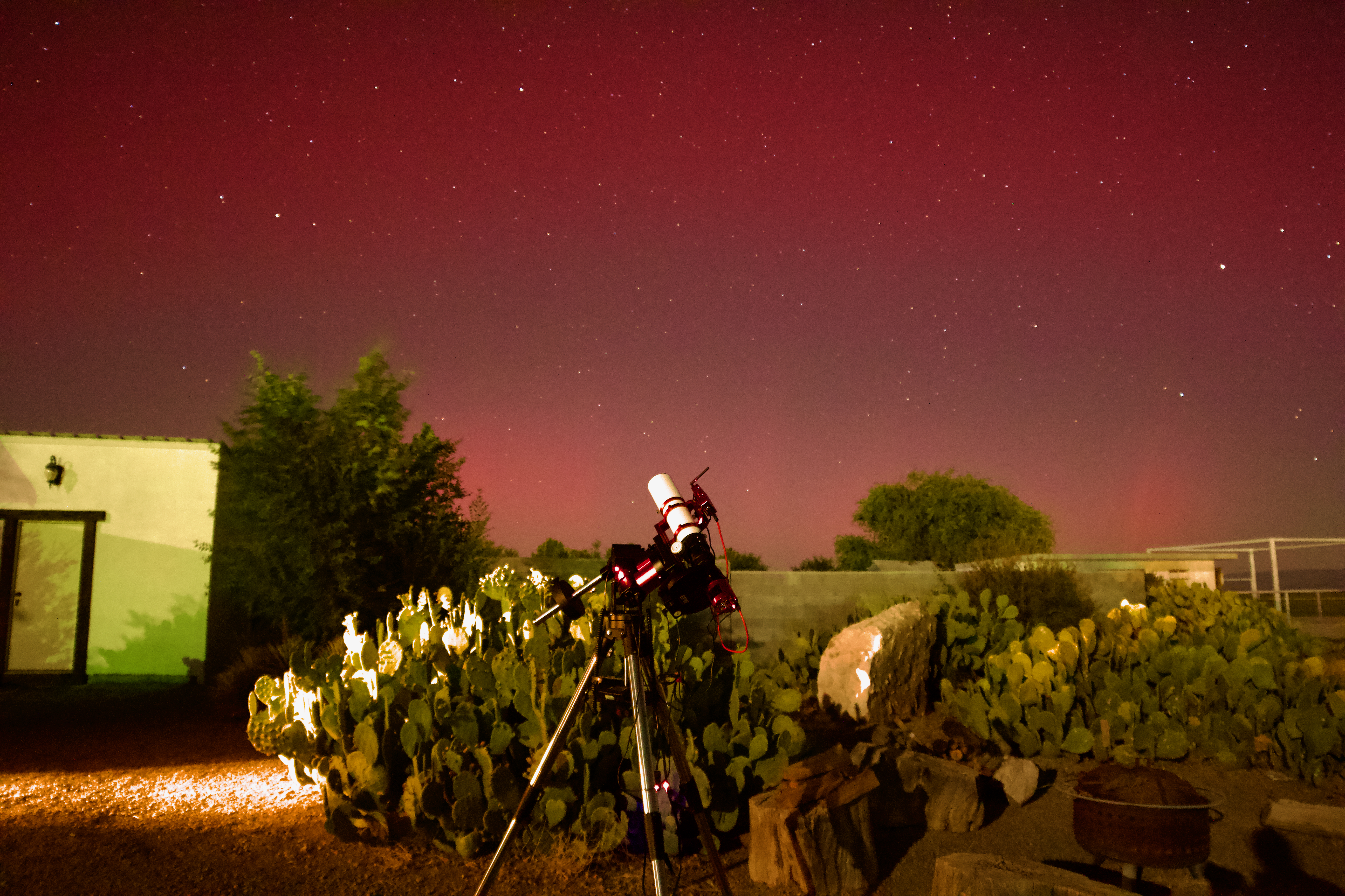
I took glamour shots of our Air B&B with the aurora.
I made some time lapse movies.
Camera geek info:
And I’m left with the question: when can we see this again? It was amazing.
What amazing things have you seen recently?

I was looking through my comet posts after my post yesterday, and I discovered I hadn’t posted this image of Comet PANSTARRS C/2021 S3 with two globular clusters that I made last spring. Enjoy!
I hadn’t planned on imaging comets when we were in Dell City last spring, but when I saw this combination of two globular clusters and comet PANSTARRS C/2021 S3, I knew I had to try it.
Globular cluster M9, the brighter one to the left, is 25,800 light years away from us. It’s 90 light years across, giving it an apparent size of 12 arcminutes. Globular cluster NGC6356, the smaller one to the right, is 49,200 light years away from us. Its apparent diameter is 8 arcminutes, giving it a diameter of 115 light years across. Globular clusters are mind-bogglingly old parts of our galaxy and can be used to infer the age of the universe. There are some interesting open questions about them, including their exact ages and whether they formed as part of our galaxy or were accreted later (probably a mix of both). In the paper I found giving the ages for these two globular clusters, it shows that M9 is 14.60 ± 0.22 billion years old with one model, 14.12 ± 0.26 billion years old with a second model, and 12 billion years old in the literature. It shows that NGC6356 is 11.35 ± 0.41 billion years old with one model, 13.14 ± 0.64 billion years old with a second model, and 10 billion years old in the literature. No matter which age ends up being correct, ~10 billion years old is amazingly OLD!
Comet PANSTARRS C/2021 S3 was discovered by the Panoramic Survey Telescope and Rapid Response System located at Haleakala Observatory, Hawaii on images taken on September 24, 2021. It reached perihelion (its closest point to the sun) on February 14, 2024 (the day after this image was taken) at 1.32 AU distance. Its orbital eccentricity is higher than 1, meaning it’s on a parabolic trajectory and isn’t coming back.
I feel very fortunate that my trip out to the dark skies was timed so I could image this comet with two ancient globular clusters. I also feel fortunate that I imaged it in a time when so many processing tools are being developed to make processing the image so much easier! The tools I have this year are so much more powerful than the ones I had last year.
Camera geek info:
Frames:
Processing geek info:
