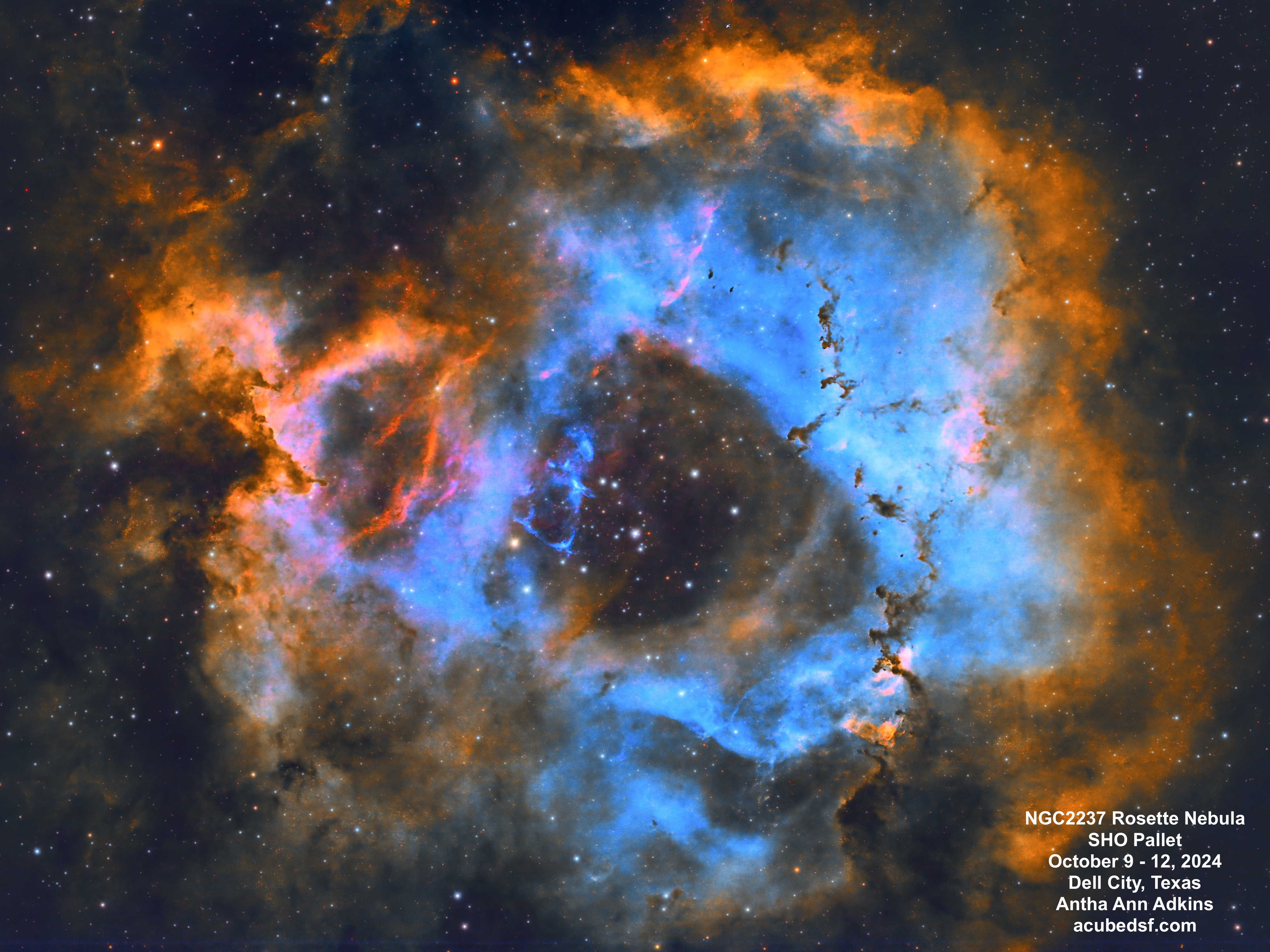
Usually I don’t image on work nights so I get enough sleep.
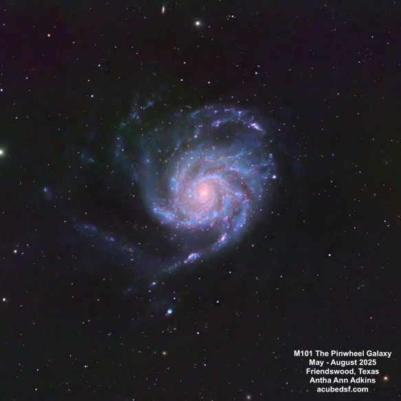
However, the new telescope cloud curse has been strong, and I’ve only had a few clear nights since I bought my new William Optics Pleiades 111 telescope “Blue” earlier this year. So when it was finally clear on Tuesday, I couldn’t resist taking my new telescope outside. I continued to collect data on M101, but I had learned through a Facebook post that there was a new supernova in the galaxy NGC7331. So after M101 set, I spent the rest of the night imaging NGC7331.
NGC7331 is an unbarred spiral galaxy. It’s located approximately 47 million light years away, and it has an apparent size of 10.47 arcminutes, making it about 144 thousand light years across. One paper on this galaxy argues that its central bulge rotates in the opposite direction of its outer disk – weird! Another argues that the stars in the central bulge are old – 13 billion years old, while the stars in the disk are young – possibly 0.2 billion years old. (This may not be unusual; our own galaxy is still making stars in its outer arms right now, which I also think is really cool.)
Supernova 2025rbs is a Type 1A supernova, which occurs when a white dwarf star collects material from a companion star, almost reaches the Chandrasekar mass, starts fusing carbon, experiences a runaway reaction, and explodes, releasing an enormous, but predictable, amount of energy. Type 1A supernovas can be used as standard candles to measure the distance to the supernova (and in cases like SN2025rbs the distance to the home galaxy) because the energy they release and thus their brightness is predictable. SN2025rbs was discovered by the Gravitational-wave Optical Transient Observer (GOTO) on July 14, 2025.
You can clearly see SN2025rbs as a bright spot near the galaxy center. In fact, it appears to outshine the galaxy center, which I find amazing.
When I imaged this, I deliberately used short capture times (15 seconds) so that the bright supernova would not “blow out” and clip to pure white or cause “pixel bloom” where the light overwhelms the pixel capturing it and so bleeds into the nearby pixels.
I spent a fair bit of time thinking about how this image “should” be processed. On the one hand, I wanted to preserve the relative amount of light and color for the supernova relative to both the star field and NGC7331, its host galaxy. On the other hand, astroimages are inherently low-light and high dynamic range, which means that the data has to be non-linearly stretched to show both the relatively bright supernova and stars and the relatively dim galaxy.
My standard PinInsight processing flow includes using BlurXTerminator (BXT) to sharpen the stars and non-stellar objects, NoiseXTerminator (NXT) to remove noise, and then StarXTerminator (SXT) to separate the stars from the non-stellar objects so they can be stretched separately.
I considered whether I should skip the BXT processing step. BXT sharpens the stars and makes them smaller, and it did the same to the supernova but not the NGC7331 galactic core. The BXT documentation says, “BlurXTerminator is trained to conserve flux, the total amount of light associated with a feature such as a star. When a blurred star is made less blurry, the light from some number of pixels is concentrated into a smaller number of pixels. Those pixels must get brighter for the total amount of flux to be the same.” Based on that statement, I think since BXT preserves the amount of light in each star, it also preserves the relative amount of light between the stars and between the stars and the supernova (assuming none of them are clipped because they exceed the max brightness level, which did not happen in this case). Further, since stars (and supernovae) are point sources of light and with perfect seeing and optics would only be “seen” in one pixel, using BXT to sharpen the stars and the supernova should be making them more like their “true” amount of light relative to the galaxy as well. So I left the BXT step in my processing flow.
I also considered whether I should skip the SXT step and stretch the stars, supernova, and galaxies together or use SXT and stretch them separately. Either way, there is no longer a linear relationship between the brightness of the objects. If I processed this as a single image, the brightness ordering – what is brighter than what – would be maintained. If I used SXT so I could stretch the galaxies separately, I could end up making the galaxy core brighter than the supernova, even though it was not in the raw data. On the other hand, I could show more detail in the galaxy if I processed it separately. I ended up deciding that, in this case, what was most important to me was to maintain the brightness order and show that the supernova was brighter than the galactic core. So I processed it as a single image.
My final PixInsight processing flow was:
- WBPP to calibrate, normalize, and integrate three channels of RGB data
- ChannelCombination to combine the RGB channels into a single image
- DBE to remove the excess blue in the background
- SPCC to calibrate the color
- BXT to sharpen the stars and the galaxy
- NXT to to remove some noise since this is only a few hours worth of data from my Bortle 7-8 light polluted skies
- Histogram Transformation to stretch the image
At some point, I’d like to collect more data on this galaxy and make a nicer picture of it. But the clouds are back now. The curse continues …
Camera geek info:
- William Optics Pleiades 111 telescope
- ZWO 2” Electronic Filter Wheel
- Antila RGB filters
- Blue Fireball 360° Camera Angle Adjuster/Rotator
- ZWO ASI183MM-Pro-Mono camera
- William Optics Uniguide 32MM F/3.75
- ZWO ASI220MM-mini
- ZWO ASiair Plus
- iOptron CEM40
- Friendswood, Texas Bortle 7-8 suburban skies
Frames:
- Lights
- 248 15 second Gain 150 Red lights (62 minutes)
- 182 15 second Gain 150 Green lights (45.5 minutes)
- 168 15 second Gain 150 Blue lights (42 minutes)
- 30 0.2 second Gain 150 Red flats
- 30 0.1 second Gain 150 Green flats
- 30 0.1 second Gain 150 Blue flats
- Darks, Flat darks from library